BlueDot Technical AI Safety Puzzle #1 - Submission

Full experiment code: tasks 1 and 2 · task 3 · trained model (also available in task 3)

About me: I have been coding my entire life, I’ve never finished college (or high school for that matter). I trained a “few” deep-learning models over a 10-year career as a backend developer and am now transitioning full time into AI safety research. Some of my approaches may look stupid or unnecessarily complex/trivial to someone who knows more math and/or ML theory and doesn’t need to run an experiment to know how it will end, it is what it is. This puzzle was a lot of fun, thank you for creating it! Special thanks to Zuzanna Matuszewska from AI Safety Poland for showing me the puzzle and pushing me to give it a try.

Short description of the puzzle

Model is a frozen MiniLM sentence encoder (a pre-trained model that turns a written sentence into a list of numbers) followed by a small trained head that predicts eight yes/no features of each sentence (country, food, sentiment, and five others that do not matter for the sake of the puzzle).

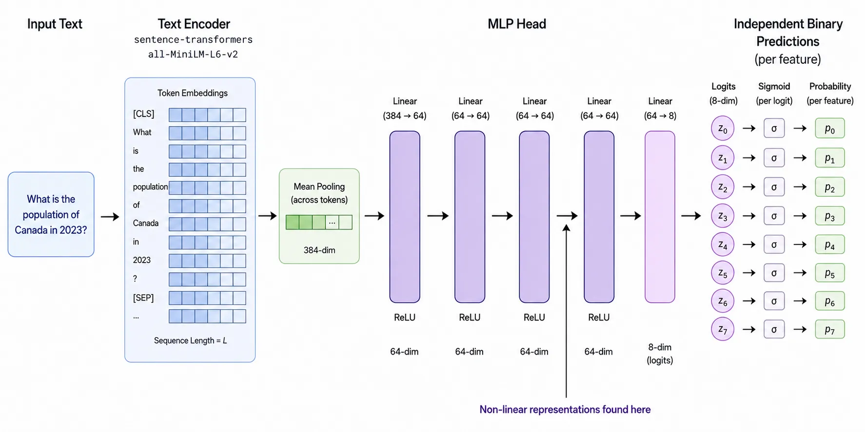
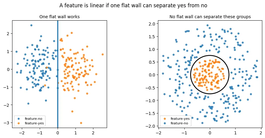
At layer L each sentence has been turned into a list of 64 numbers, so each sentence is a single point in a 64-dimensional space. Inside this space, seven of the features are linear (can be predicted by linear regression) and one is not. The goal is to find the one that is not and explain how it is represented in the output of layer L. If we were 64-dimensional beings, we could simply look at the shape each feature makes. Well I can’t, because 64 is slightly more than 3 (which I am barely comfortable with), so most of the solution is about building a plot we can look at and think about.

Solution to the puzzle

answer to task 1

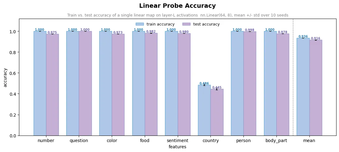
The weirdly represented (nonlinear) feature F is country. I trained one linear layer trying to predict all features at once from the layer L activations, retrained 10 times with different random seeds. Seven features are predicted with ~0.97–1.00 accuracy while country sits at ~0.445, below random chance. Since original model predicts country with accuracy of ~0.964 the information has to be there, just stored in a shape the probe can’t read.

short answer to task 2, long answer below

At layer L, country is represented mainly by distance from the center of a 2D plane hidden inside the 64-dimensional activation space. Country sentences lie near the center, while non-country sentences lie farther out. Due to that, linear probe cannot isolate this central bullseye from the surrounding points.

Task 2: how country is represented

Cutting dimensions away

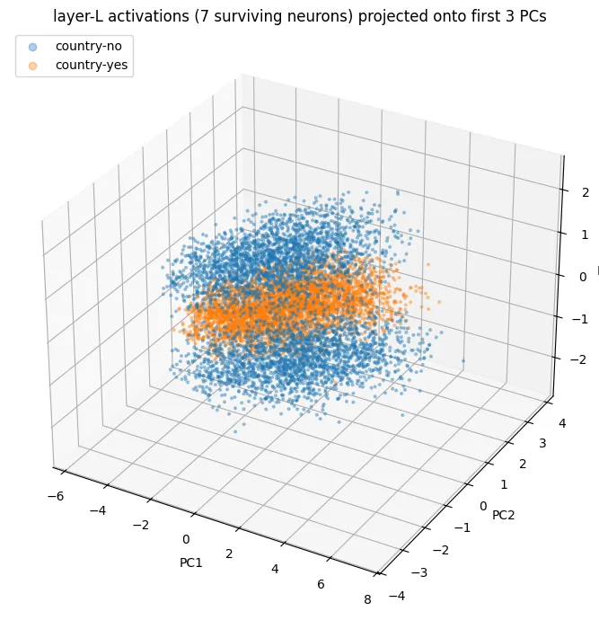
To understand layer L activation structure I wanted to reduce dimensionality of the layer L activations as much as possible, so I can literally look at the geometry of the solution myself. My first attempt was a probe that pays an extra loss for every neuron it uses (I later learned this is a naive version of sparse probing); this probe, like the other more advanced probes below, is a small neural network that can learn nonlinear boundaries. It turned out that 7 neurons predict country at 96.3% ± 0.5%, practically matching a probe that uses all 64 (96.7%).

Seven dimensions is still more than three, I had no idea how to look at the structure without reducing it further, I found two methods for that:

Principal Component Analysis is a go-to method that shows the most overall spread (or variance) in the data. It gave the first visual I could look at, but the picture was a weird blob that didn’t have enough structure and didn’t convince me to be final solution to the puzzle. It took me a while to figure out, but the reason why is that the other seven features share the space and have their own spread, so PCA has no reason to give a clean view of country specifically.

After that I let gradient descent choose the linear projection angle instead. I trained a bottleneck probe that squeezes the 64 numbers through a learned projection down to just k dimensions and must predict country from those k alone. If accuracy stays high at small k, the whole structure fits in a picture with k axes. k=2 already reaches 0.973, matching the full 64-neuron probe (0.967): That means that all the country feature information can be compressed into a flat 2D plane.

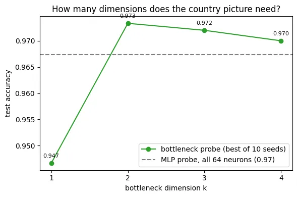
What first weirded me out was that k=1 already scores 0.947, but this is just what a dartboard looks like when you view it edge-on: the bullseye becomes a segment in the middle of a line.

The bullseye

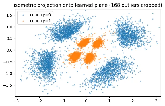
The learned projection is allowed to stretch and skew its picture (its two raw axes met at 61° and had unequal lengths), so before trusting any distances I corrected the view to keep same distance in every direction (a QR orthonormalization). After plotting our points, we finally have a first solid 2D view of the structure: country=1 sentences form four small blobs inside a central region, and country=0 sentences are a little bit further behind them.

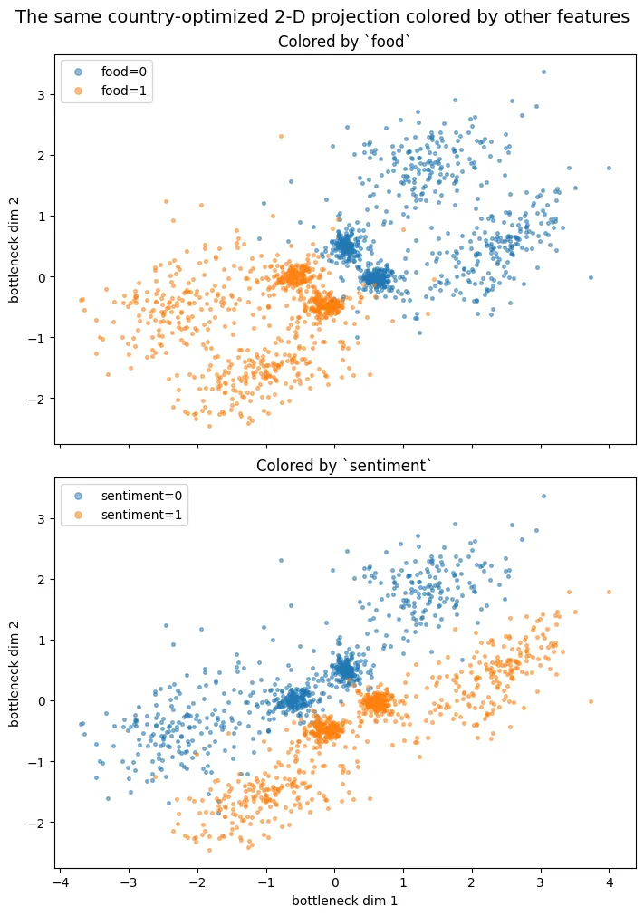
Coloring the plot by the other seven features helps to understand the blobs, the plane works like a dartboard. Direction from the center encodes the food/sentiment combination and the distance from the center encodes country. I ran a few checks: predicting from the direction alone reads food at 0.983 and sentiment at 0.980, while country from the direction alone is 0.463, which is random and shows that distance and angle of the dartboard encode different information.

Does the model actually use the radius?

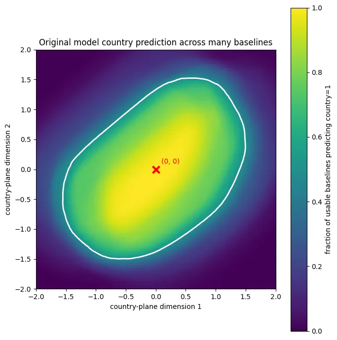
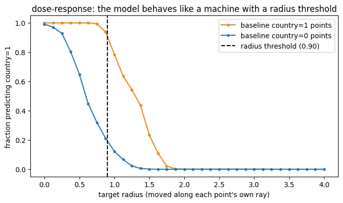
The bullseye could be only a correlation found by the probe. To test whether the model itself actually uses it, I edited the layer-L activations and measured how the original model’s predictions changed. Each 64-dimensional activation can be split into two parts: its position in the 2D plane and the remaining 62 dimensions outside that plane. I placed activations at different positions across the plane while keeping their other 62 dimensions fixed. The model predicts country=1 inside an elliptical region around the center and country=0 outside it. This boundary comes directly from the original model.

Next, I moved each sentence toward or away from the center while keeping its direction and other 62 dimensions unchanged. Moving country=0 sentences inward flipped the country prediction 82.1% of the time. Moving country=1 sentences outward flipped it 99.2% of the time.

The other seven predictions changed in only 0.6-1.2% of cases. Changing the radius changes almost only the country prediction.

Does the model use this plane?

The dartboard came from the highest-accuracy bottleneck probe and this creates a potential problem: the probe found a plane from which country can be decoded, but that may or may not be the plane the model itself uses.

To find the model plane, I computed the gradient of its country output with respect to the 64 layer-L activations. For each sentence, this gradient points in the direction that would change the model’s answer fastest. This requires neither another probe nor the true labels. Across sentences, 97.3% of the variation in these gradients lies in just two dimensions. The model’s sensitivity to country is itself ~entirely 2D.

The probe plane also aligns strongly with this gradient plane. Their overlap is 0.757, where 1 means identical planes and random 2D planes in 64 dimensions score about 0.18. This also explains the differences between probe seeds: the best probes overlap the gradient plane by 0.68-0.76, while the weaker probes score around 0.33. Weaker probes found tilted views containing only part of the signal.

As a last sanity check I tested whether the plane is necessary. I replaced every test sentence’s position in the probe plane with the same average position, while leaving the other 62 dimensions unchanged. country accuracy fell to 0.501, while the other seven features lost at most about two percentage points so we know that no usable copy of country remains outside the plane.

How does linear representation of the country disappear and how does it return?

To understand fully how that happens, I set up linear probes across the network to show exactly where the feature is recoverable by a linear probe and where it is not.

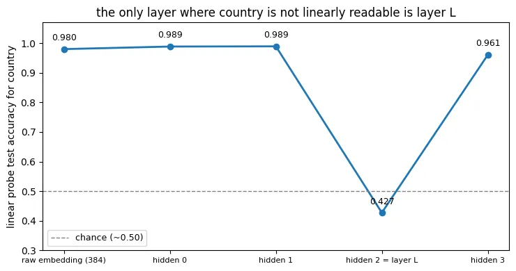
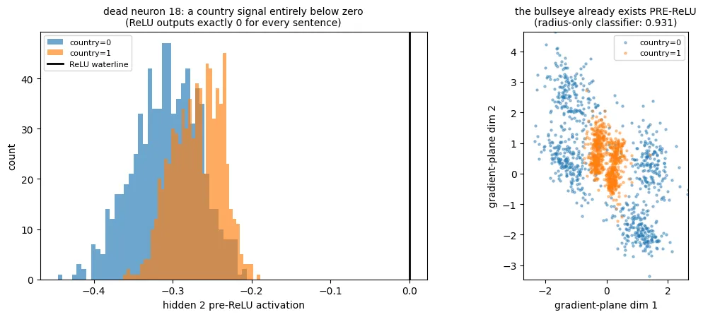
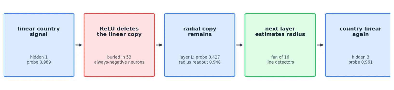
Before layer L’s activation, linear probe still reads country well. However, almost all of that signal is stored in 53 neurons whose values are negative for nearly every sentence. Those neurons (tested linearly) alone reach 0.981 accuracy, while the remaining 11 reach only 0.476. The ReLU sets all negative values to zero, so it deletes the linear copy of country in a single step. The transformation from hidden 1 to these activations is linear, so it can rotate or stretch an existing geometry, but it cannot create a new nonlinear interaction. Hidden 1 therefore already contains both a linear copy of country and a radial one. Layer L removes the linear copy, leaving only the bullseye. This is verified directly in the notebook: classifying by distance from the bullseye center already works on the pre-ReLU values (0.931, vs 0.948 after the ReLU), so the radial copy exists before the ReLU fires and the only thing the ReLU deletes is the linear copy.

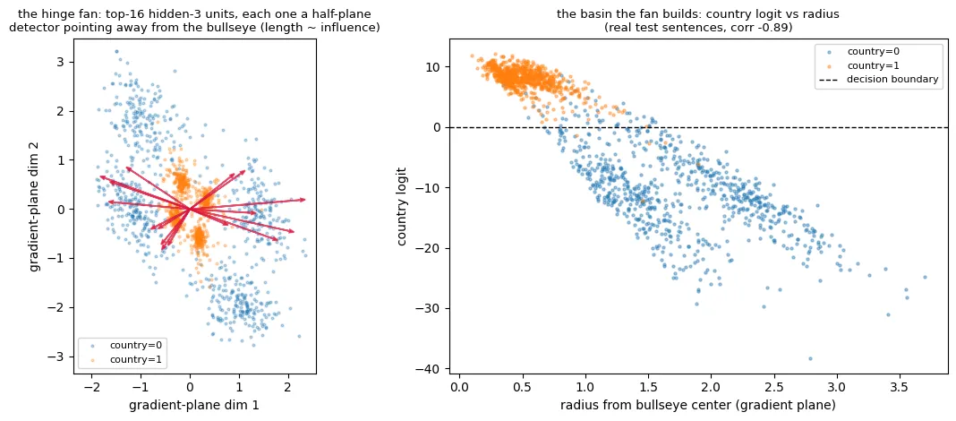
The next layer converts radius back into a linear signal using a fan of line detectors. Its 16 most important country units all work in roughly the same way: each draws a line across the 2D plane, stays inactive on one side, and becomes increasingly active as a point moves across the line. Their lines face outward in different directions around the bullseye. When their outputs are added together, they approximate distance from the center, allowing for the linear readout from that signal. What’s interesting is that the detectors are also distributed unevenly around the plane, making the decision border more of an ellipse than a circle.

I’d expect that behavior to be explicitly trained into the network using some adversarial training to make country difficult for a linear probe exactly at layer L.

Task 3: weirder representation of country

The original model always stores country in the same geometric structure, a fixed 2D plane where distance from the center determines the answer. I trained a model whose decoding rule depends on the input itself.

Locker code

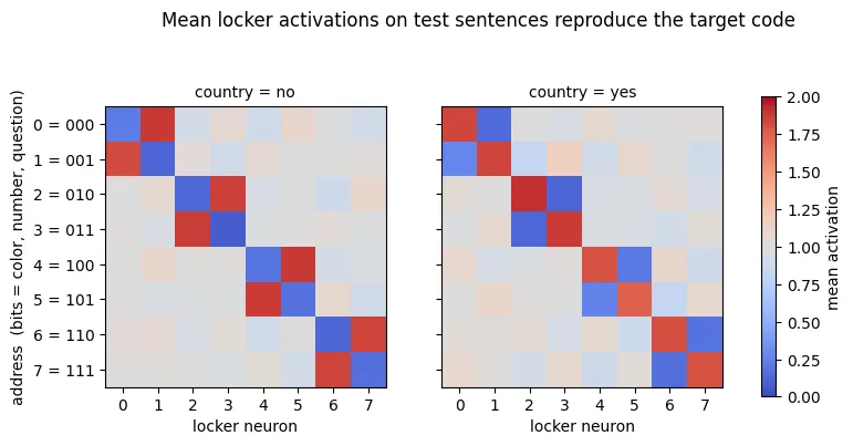
The model uses 8 of the 64 layer-L neurons as “lockers”. Three other binary features, question, number, and color, form a 3-bit address that selects one of those lockers.

The selected locker stores the country bit, its paired locker stores the opposite value, and the other lockers remain neutral, two sentences with the same country label may store it in completely different neurons.

Single “country neuron” or fixed direction to inspect doesn’t exist and decoder must learn how to read the three address features and only then it can know which locker contains the answer.

Training

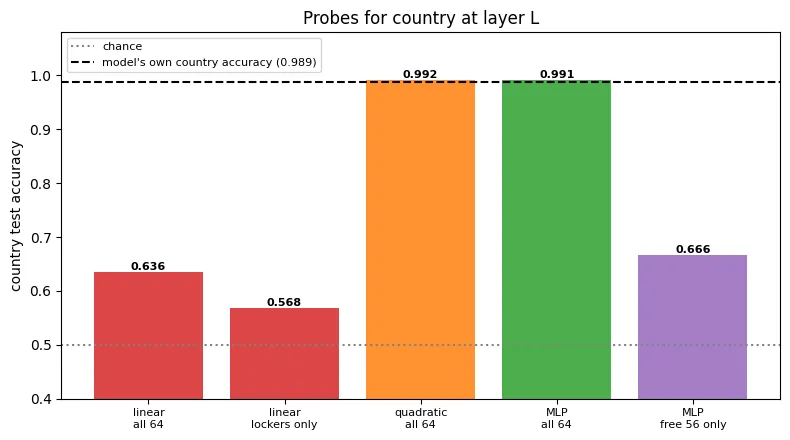
I used the same data, frozen encoder, and model architecture as in the original puzzle. Training had three goals: keep original prediction accuracy, make the lockers follow the intended code and prevent the model from keeping a readable copy of country elsewhere in layer L (even an MLP probe on the 56 non-locker neurons reaches only 0.666).

If we ablate any of these conditions, model is unable to learn the task while maintaining nonlinearity. Earlier versions learned the locker code but also stored nonlinear copies in the remaining neurons. I fixed it with training adversarial probes alongside the model to remove the copies.

I tested several code sizes and selected 8 lockers because it was the largest version that trained well while being used by the model to make the prediction.

Results

The weirded model remains accurate, country accuracy is 0.989 and all eight features score at least 0.945. Linear probe on all 64 layer-L neurons can reach only 0.636 and at the same time locker contains the correct bit for 99.0% of the test sentences.

I ran causal interventions to show that the model actually uses the learned code. Rewriting the locker pair flips model country prediction 94.5% of the time, while if we force every locker to its neutral value crushes accuracy to 0.503 and this ablation six of the other seven features are almost unchanged (as a training artifact, part of body_part is stored inside the locker region).

Limitations

This representation doesn’t defeat every simple probe. Quadratic probe can still decode country with about 0.99 accuracy. The model also doesn’t dereference the selected locker perfectly: rewriting a random non-addressed pair flips the country prediction 28.7% of the time.